Improved Approximation Algorithms for Maximum Cut and Satisfiability Problems Using Semidefinite Programming (Michael X. Coemans and David P. Williamso, 1994) reading note.
Introduction
Defn (Maximum Cut Problem): Let G=(V,E,w) be a undirected graph with weigh function w:E→R. One wants a subset S of the vertex set V such that the sum of the weights of the edges between S and the complementary subset S is as large as possible.
The maximum cut problem can be written in the following integer programming form:
max s.t. 21i<j∑(1−xixj)wijxi∈{−1,1}, i=1,2,…,n(1)
However, maximum cut problem is a NP-complete problem, which means that it probably has no polynomial time algorithm.
Thus we try to find its approximate solution.
Relaxation
Since solving (1) is NP-complete, we consider semidefinite relaxation of (1).
xi∈{−1,1}=S1⟹vi∈Sn,
where Sk denotes the k-dimensional unit sphere.
Then we can write down the semidefinite relaxation of (1):
max s.t. 21i<j∑(1−Xij)wijvi∈Sn, i=1,2,…,nXij=⟨vi,vj⟩, i=1,2,…,n, j=1,2,…,n(2)
Thm: X is a semidefinite matrix. Thus problem (2) is a semidefinite programming problem.
Proof: For every y∈Rn, we have: \vspace{-0.3cm}
yTXy=i,j∑yiyj⟨vi,vj⟩=i,j∑⟨yivi,yjvj⟩=⟨i∑yivi,i∑yivi⟩≥0,
as desired. □
Algorithm
Then there is a simple randomized approximation algorithm for the maximum cut problem.
- Solve (2), obtaining an optimal set of vectors vi.
- Let r be a vector uniformly distributed on the unit sphere Sn.
- Set S={i∣⟨vi,r⟩≥0}.
Remark: We can obtain {v1,…,vn} from X by Cholesky decomposition, i.e. X=LTL and each column of L is a vi.
Analysis
We analyze the approximate effect of the algorithm:
E[w(S,S)]≜E[Δ]=i<j∑wijPr[sgn(⟨vi,r⟩)=sgn(⟨vj,r⟩)]=i<j∑wij2π2arccos(⟨vi,vj⟩)
Then let p∗ be the optimal value of problem (1), and q∗ be the optimal value of problem (2).
Since (2) is a relaxation of (1), we have that q∗≥p∗. Thus the approximation ratio p∗E[Δ]≥q∗E[Δ].
If wij≥0 for every i,j, then we have:
q∗E[Δ]=π2⋅∑i<jwij(1−⟨vi,vj⟩)∑i<jwijarccos(⟨vi,vj⟩)≥π2i,jmin1−⟨vi,vj⟩arccos(⟨vi,vj⟩)≥π2θmin1−cos(θ)θ≜α≈0.878…
Remark: By using Markov inequality and the fact E[(p∗−Δ)/p∗]<0.122, we have:
Pr[(p∗−Δ)/p∗>0.122ϵ]<1+ϵE[(p∗−Δ)/p∗>0.122ϵ]<1+ϵ1<1
We can repeat this algorithm many times to reduce the error probability.
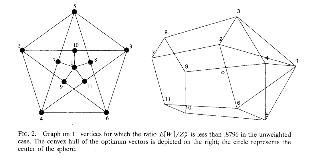
Quality of the Relaxation
The following picture shows that the bound showed before is almostly tight.
Analysis for Negative Edge Weights
For negative edge weights, we have:
Thm: Let W−=∑i<jmin{wij,0}. Then:
E[Δ]−W−≥α(q∗−W−)
The proof of this theorem is almostly the same as before.
Supplements
- The maximum cut problem is APX-hard, meaning that there is no polynomial time approximation scheme, arbitrarily close to the optimal solution, for it, unless P=NP.
- If the unique games conjecture is true, this is the best possible approximation ratio for maximum cut. (Subhash Khot, Guy Kindler, Elchanan Mossel and Ryan O’Donnell, 2004)
Thm (Unique Games Conjecture): Given any ϵ,δ>0, there exists some k>0 depending on ϵ and δ, such that for the unique games problem with a universe of size k, it is NP-hard to distinguish between instances in which at least a 1−ϵ fraction of the constraints can be satisfied, and instances in which at most a δ fraction of the constraints can be satisfied.
Further statements about UGC can be seen on https://www.zhihu.com/question/264803851
References
[1] Michel X. Goemans and David P. Williamson. 1995. “Improved approximation algorithms for maximum cut and satisfiability problems using semidefinite programming.” J. ACM 42, 6 (Nov. 1995), 1115–1145.
[2] Lecture 3 of the course Algorithms for Big Data, 2024 spring, lecturer: Hu Ding and Qi Song.
[3] Subhash Khot, Guy Kindler, Elchanan Mossel and Ryan O’Donnell. “Optimal inapproximability results for MAX-CUT and other 2-variable CSPs?.” SIAM Journal on Computing 37.1 (2007): 319-357.